Introduction to Digital Images
Written September 8th, 2021
Images, etc
Images are, of course, sets of visual data. With any sort of processing, it is important to differentiate between analog and digital types. Analog images are real life things such as photographs, paintings, medical images, et cetera. So then, digital images are things like .pngs, .jpgs, and so on (while these are usually called "photos" it is important to state their explicit name so not to confuse them). We can explicitly represent images mathematically by a function I(x, y).
I(x, y) is a function in which x represents the horizontal spatial dimension and y represents the vertical spatial dimension. Thus, the units are some form of length. Videos would add a time component to this. The function I(x, y) is a continuous function that, for our purposes, is sampled at regular intervals to produce a digital image. This sampling is best represented as pixels per inch (PPI). A PPI of 2000 means that an analog image is sampled 2000 times in one inch. For a 1" by 1" square, this would mean there are 10002 samples.

The equation above is the full representation of a digital image. The image consists of M rows and N columns where any arbitrary location can be found between 1 ≤ m ≤ M and 1 ≤ n ≤ N. The values T1 is the sampling distance (inverse of the sampling rate such as PPI) in the horizontal direction and T2 is the sampling distance in the vertical direction. Combined, these all form the pixel (short for picture element) that is I[m, n].
Monochromatic images are typically displayed in grayscale which ranges from white to black in intensity. A sampled grayscale image would be represented as a two-dimensional array of numbers I[m, n]. For most digital images, the value of I[m, n] at any given point is always positive and finite. E.g:

This bounding of the function is from the physical nature of the image; it doesn't make sense to have an infinitely intense physical value of light. One's monitor wouldn't be able to reproduce it nor would a computer be able to store it. The bound at Imax comes from the storage of the data on the computer. This allows the intensity of the image to be relative to a certain level. This is very useful for some digital signal processes that expand the range of an image's intensity, for example. Most digital images use an 8-bit intensity value. This means that Imax has a maximum of 28 - 1, or 255, creating a range from 0 to 255 with 256 distinct intensity values.
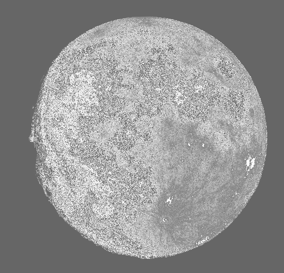
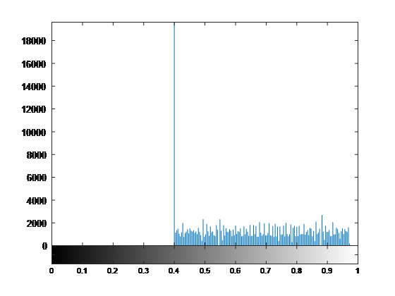
Take, for example, the image of the moon displayed below. Next to it is a histogram of how many pixels are at what intensity.
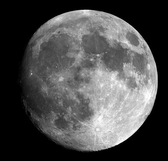
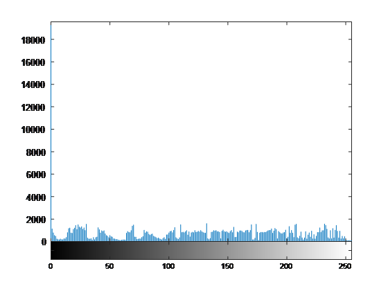
Notice all how the image has an even selection of intensity values - it doesn't favor being too bright or too dark so the image is balanced or equalized adequately well. If an image isn't balanced well, it's said to have a low contrast. Low contrast is usually hard for us with human eyes to see, and equally as difficult for digital image processors to make use of. While this image has rather well contrast width, it could be a bit better equalized due to the value of intensities at r = 0. Now we need to start thinking in terms of transformations to improve the contrast equalization.
Transformations
The most generic and arbitrary transformation is a mapping function z = T(r) where r is the input intensity and z is the output intensity at any given pixel at location [m, n]. There is generally no restriction to the transformation T other than it must be defined within the working range of the intensities r and z. One very common type of transformation is a thresholding function where the graph of z(r) is split into two distinct regions of r. Two points are defined at (r1, z1) and (r2, z2). If z1 = 0, z2 = L - 1 (where L is 2# of bits), and r1 = r2. This results in the shape of the graph given here (desmos link). What this function does is it ignores any data below a certain input intensity (T(r) = 0) and intensifies any data above a certain intensity (T(r) = L - 1).
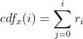
Another type of contrast stretching is histogram equalization. I know MATLAB has this function already available, but it's worth going into what exactly histogram equalization does. The first new function I must introduce is the Cumulative Distribution Function (CDF). This function is a summation of the number of pixels at each intensity. The explicit definition of the CDF is displayed below. Here is also a link to the wikipedia article.
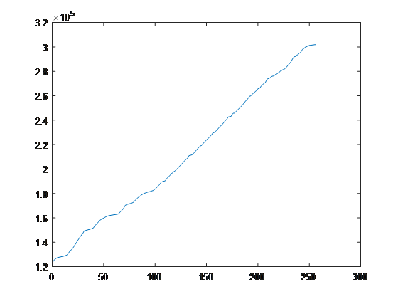
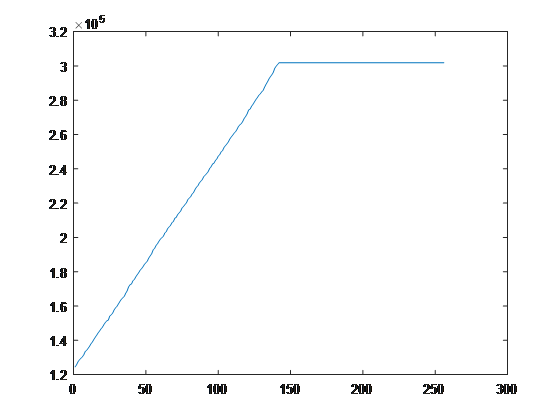
The CDF of an image always sums up to equal the number of pixels in the image. For a 3x3, 2-bit intensity image with 6 black (intensity is zero) and 3 white (intensity is 3) pixels, the CDF would be [6, 0, 0, 3]. Notice how the CDF is a length of four, which corresponds to the 2-bit resolution (22 levels of intensity). With this function in mind, the CDF of the moon image is displayed below. One important thing to take notice of is the vertical axis of the graph - it doesn't start at r0 = 0 - but rather r0 ~= 1.2E5. This means that the lower intensity values are heavily favored in the image. We can clearly see this with the black background of the original moon.png image.
This CDF is our transformation T(r). This can be explained conceptually. We want to even out the full range of an image so that each intensity has an equal part in the image intensity histogram. So, if there is a spike in low intensities (like our case), then we should prioritize the high intensities so that the high intensities have equal footing. We know our image has an equalized histogram when the image post-transformation results in a CDF that is representative of a linear function as close as possible. (An example of this is under "full-sized image" on the wikipedia page). After normalizing the CDF for the moon image, below is what the transformation did to the image along with the intensity histogram and the CDF itself.
Sadly, the image loses some contrast width when we put it through this function, but the function did exactly what we wanted it to do. It equalized the intensity histogram and made the CDF as linear as possible. (Also, the image did decide to die a bit as I put it through my processor, I wonder where this bug lies within MATLAB).